Investigating a social network using Graph Theory
This project will investigate a social network using graph theory. The first part of this project will find a dominating set of users in a network (i.e. users with at least one connection to all the other users in the network). The second part of the project will find sub-communities or tightly connected communities within a network
The data used will be the provided Facebook datasets facebook_1000.txt, facebook_2000.txt and facebook_ucsd.txt
facebook_1000.txt has 783 vertices (persons) and 3784 edges (friendships).
facebook_2000.txt has 1780 vertices (persons) and 15,650 edges (friendships)
facebook_ucsd.txt has 14948 vertices (persons) and 886442 edges (friendships)
Note: The above datasets is slightly different from what was given in the initial proposal.
For answering the easier question (dominating set) the facebook_1000 and facebook_ucsd datasets will be used. For answering the harder question (finding sub-communities the facebook_1000 and facebook_2000 datasets will be used.
Easier: To find the dominating set of nodes in a Facebook network. A dominating set is defined as the subset of users who are connected to all the users in the network. This is useful for marketing messages or targeting “super” users or influencers in a network.
Harder: To find sub-communities in a Facebook network. Sub-communities are closely connected users who interact with each other more and share certain commonalities like same high school or same subject interest etc.
The graphs are visualized using GraphStream package (http://graphstream-project.org)
The network was laid as a classic graph data structure using an adjacency list. Each person is denoted as a vertex and a friendship is denoted as an edge in the graph.
A HashMap of integer key to denote a vertex and HashSet of integers for its value to denote edges was used.
Although having this data-structure had its limitations (for example to find an edge which had the vertex as an end node), it was sufficient to answer this question as the algorithm was less complicated. See below for the data structures used to answer the harder question.
The algorithm used was the one laid out in the project idea: Broadcasting to a twitter network lecture. The outline of the algorithm is as follows:
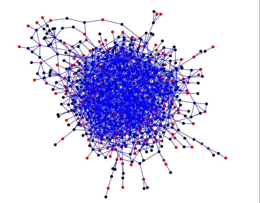
The dominating set for the final run using the facebook_1000 dataset is shown below. For a network size of 783 vertices and 3784 edges, a dominating set of 266 vertices were found. Dominating set of vertices are in red and all the other vertices are in black.
For the facebook_ucsd dataset (size of 14948 vertices and 886442 edges) a dominating set of 2546 vertices were found. The graph is not displayed here as the image was too cluttered and visually not intuitive.
The network was laid as a classic graph data structure using an adjacency list. Each person is denoted as a vertex and a friendship is denoted as an edge in the graph.
A HashMap with the user id as an Integer key and Node object as the value was created.
A HashSet of edges (denoting friendship connections) was also maintained in the program.
Each Node object had a HashSet of edges within it in addition to the actual user id (stored as an integer). Each edge object pointed to the nodes that it connected.
This data-structure made more sense than the simple HashMap<Integer,HashSet<Integer>> data-structure that was used to answer the easier question above. The addVertex and addEdge methods were modified to incorporate both types of data-structures to make the code compatible for answering both questions.
The algorithm used was the one described in the project ideas lecture: Detecting communities This algorithm is formally known as the Girvan-Newman algorithm
The steps in the algorithm are as follows:
To measure the betweenness of each edge a modified version of the Brandes algorithm for finding betweenness centrality of each vertex was used.
The Brandes algorithm is as follows:
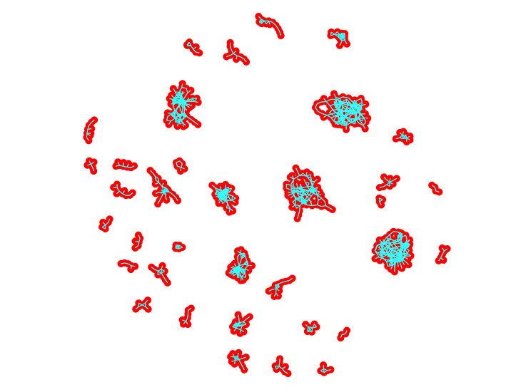
For the facebook_1000 dataset (size of 783 vertices and 3784 edges), by achieving a max edge betweenness score less than 500, we get the output as shown below
Number of sub-communities detected = 35
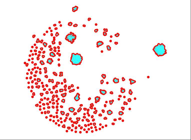
For the facebook_2000 dataset (size of 1780 Vertices and 15650 edges), to achieve a max edge betweenness score of 500 or less we get the following output:
Number of sub-communities detected = 245
Usually finding the edge betweenness would require O(V2E) time, since we have to find the shortest paths from each to every other node in that graph. Each Breadth-first search (BFS) takes O(E) time. The beauty of the Bandes algorithm is that it can do this thru a single BFS search for each vertex.
Thus the STEP1 in the code below to find the number of shortest paths takes O(E) time for an unweighted graph (refer to corollary 4 in the Brandes paper).
The STEP2 in the Brandes algorithm to accumulate the dependencies of the starting node on all the other nodes also takes O(E) time for an unweighted graph (refer to corollary 7 in the Brandes paper).
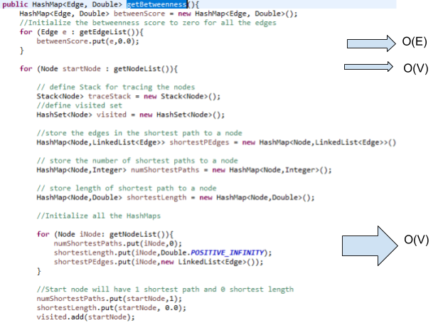
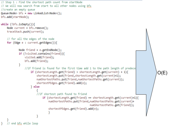
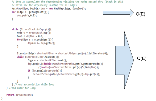
Tracing thru the actual code for the Brandes’ algorithm to find the shortest path edge betweenness. Asymptotic notation for each group of steps is shown to the right.
Adding up the runtimes we get: O(E) + O(V*(V+3E)) = O(E)+O(V2+3VE) = O(V2+3VE+E)
Since VE is the dominating term in the above equation(assuming a small number of vertices compared to the number of edges), therefore the runtime of the function is O(VE).
Since we have to run the betweenness function for every edge of the graph (removing a pair of edges with the highest betweenness in each iteration), we get a total run time of O(VE2).
The above runtime is also explained in this scholarly article on edge betweenness.
Testing was done using the dataset described in the lecture: Project Idea Broadcasting to a twitter network. The dominating set vertices are shown in red and all other vertices are in black.
Input: small_test2_graph.txt
size 8+19 Graph nodes and edges
dominating set size = 3
dominating set node 1
dominating set node 4
dominating set node 8
The above test actually shows the limitation of the algorithm (the correct set of vertices should have been 2 and 7). This is a known limitation and was discussed in the lecture (This is an approximation algorithm)
Several tests were run to verify the correctness of the code, both for step 1and both step 1 and 2. Examples were pulled from multiple lectures found on the internet. Here are some of them:
http://www.jsums.edu/nmeghanathan/files/2017/01/CSC641-Mod-4.pdf?x61976
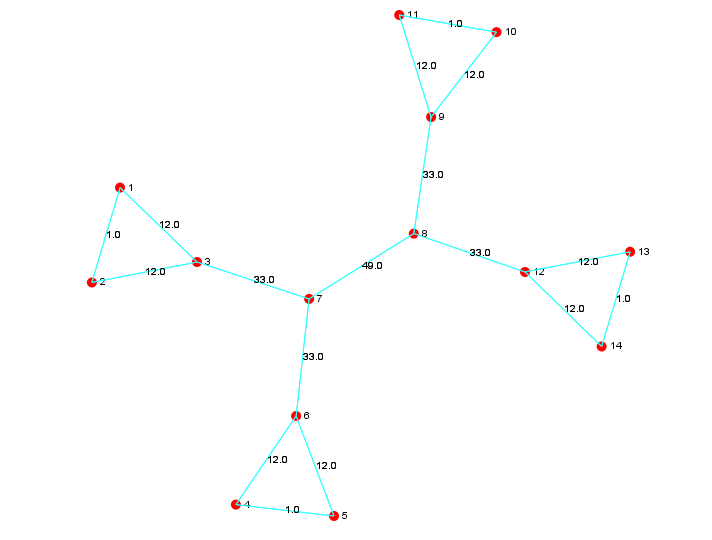
Below is an illustration of the test done with Example - 1 in the first lecture above
Highest betweenness score is for edge 7 - 8 ( and 8 -7 since this is an undirected graph)
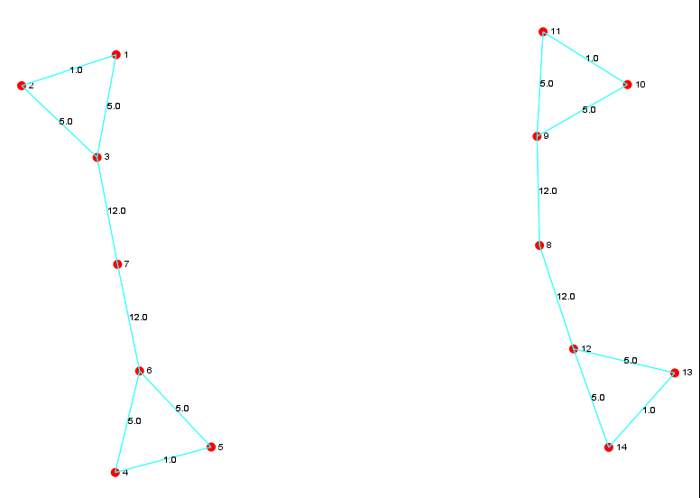
Recalculating the betweenness after iteration 1 (after removing the edges 7-8 and 8-7)
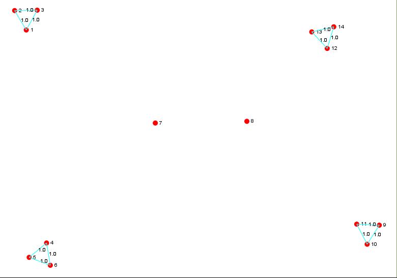
Removing the edges with the highest betweenness score (12) 3 -7, 7 - 6, 8 - 9 and 8 - 12
We end up with 4 sub-communities of vertices 1-2-3, 4-5-6, 9-10-11 and 12-13-14
For the harder question, the runtime increased quite a bit as the number of edges increased. For facebook_1000 dataset ( 783 vertices and 3784edges), the O(|V|*|E|^2) ~ 11.2 billion
To detect 35 sub-communities (betweenness score of less than 500) the process had to go thru 585 iterations. The actual run time was about 10 mins. The number of iterations was high because of multiple edges connecting the sub-communities.
For the facebook_2000 dataset (1780 vertices and 15650), O(|V|*|E|^2) ~ 436 billion (about 40 times more than the previous dataset). The actual run time was 6 hours to detect 245 sub-communities (betweenness score of less than 500)
Therefore it was not practical to run this process for the facebook_ucsd dataset which had 14,948 vertices and 886,442 edges. The big O value was 11.75 Trillion!!